Probability and Random Variables – Discrete Random Variables

Video transcript

1. Start of transcript. Skip to the end.
2. Let’s talk about discrete random variables.
3. Now, the kind of quintessential discreet random
4. variable is the value on a die when you role it.
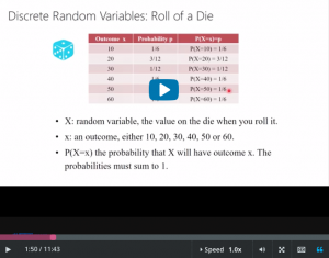
5. Now, the name of the random variable is x,
6. it’s the value of that die when you roll it.
7. Now, little x is gonna be an outcome.
8. So here it’s gonna take values either 1, 2, 3, 4, 5 or 6.
9. And then the probability that random variable X takes
10. outcome value little x Is denoted this way okay?
11. So this is the probability that random variable
12. X will have outcome little x.
13. And the probabilities have to sum to 1.
14. But for the role of a die, the outcomes are equally probable,
15. they all have probability 1/6.
16. So make sure you understand the notation here, okay?
17. So this says that the probability
18. that random variable x takes outcome 4 is 1/6th.
19. And this table is called the probability mass function.
20. It tells your for each outcome what is
21. the probability of attaining that outcome.
22. Now, here the probability mass function is constant,
23. it’s always 1/6.
24. But there are other random variables where it’s not
25. constant.
26. So here, for instance, is a PMF or a very weird die.
27. This die, instead of having values 1, 2, 3, 4, 5, for
28. 6 on its sides, it has 10,.20, 30, 40, 50, and 60.
29. And it’s also a weighted die,
30. where not all the probabilities are 1/6.
31. So here, one of the probabilities is 3/12 and
32. another is 1/12.
33. So just double check for yourself that the probabilities
34. all add up to 1, and it looks like they do.
35. Well, okay, so let’s go back and review the general notation.
36. So the random variable is called capital X, okay, and
37. the possible outcomes are called little x, and the probability
38. for outcome little x is denoted like this, okay?
39. So, this is the probability that random variable X equals
40. outcome little x, little x3, say, and that equals P3.
41. Okay, so when I’m talking about a discrete random variable,
42. I am talking about it’s PMF.
43. You cannot refer to a discrete random variable without
44. at least thinking about what its PMF is because that’s
45. what defines probability in this context.
46. Okay.
47. So, armed with this notation, let us talk about how to
48. summarize a discreet random variable.
49. Now, it’s important that when I refer to a random variable,
50. I’m referring to its probability mass function.
51. Let us talk about how one might summarize a PMF
52. without having to present the whole thing.
53. The whole thing could be very big,
54. it could be very overwhelming, and we just want one or
55. two numbers that really summarize what it looks like.
56. Okay, so how are we gonna compute the mean of the PMF,
57. mean of the random variable, and
58. how are we gonna compute the spread of it?
59. So let’s talk about the mean.
60. The mean is a measure of centrality for
61. the probability mass function.
62. What is the middle number of the PMF?
63. So we’ll use this die’s PMF, which is constant here.
64. And this is the die that
65. has the labeled sides 10, 20, 30, 40, 50, 60.
66. Okay, so what is the average outcome that you should get when
67. you roll this die over and over again?
68. And I’m sure you all know the answer, which is that it’s 35,
69. which is right in the middle there.
70. And here’s the computation you sorta did in your head in order
71. to get that.
72. You multiplied each outcome
73. by the probability that you get that outcome.
74. And then you add them all up.
75. So that’s the computation you did to get to the middle
76. number there.
77. So I can write that in general notation this way.
78. I can say that it’s outcome 1 times the probability of
79. outcome 1 plus outcome 2 times the probability of outcome 2
80. and so on.
81. And then I can write that in summation notation like this.
82. Okay, it’s the sum over i for outcome i and
83. probability of outcome i.
84. Okay, and that’s the formula for the mean of a discrete random
85. variable Okay, so let’s try this die.
86. So it’s PMF is slightly different, but
87. we can just apply the formula.
88. So it’s each outcome times its probability of occurring,
89. add them all up, and that is the mean.
90. Okay, and then here,
91. when I did that, it was a little bit less than 35.
92. And you can see why that is by looking at the probability
93. mass function.
94. See, we’ve got more mass on the smaller values here, right?
95. We moved some of the mass down lower, so we get a smaller mean.
96. Okay, so we’re now likely to choose 20 more often, so
97. that lowers the average.
98. Okay, more practice.
99. Here’s a new random variable, and here is its PMF.
100. And you can sorta look at that for
101. a bit, and realize that the values in the middle are more
102. likely than the values at the extremes, okay?
103. And you can see that from looking at these
104. numbers directly.
105. But see what if there were heck of a lot more numbers,
106. and what if the table was sort of hundreds of
107. lines longer, thousands of lines long, then you wouldn’t be
108. able to look all the numbers and figure out that some of the ones
109. in the middle are higher than the ones at the extremes.
110. Okay, so one way to handle that is to actually visualize it.
111. So I’m gonna do a bar chart of the PMF.
112. So for outcome zero, I plotted the probability to get zero.
113. For outcome 1, I plotted the probability to get 1, and so on.
114. And you can see the nice PMF without having to try and
115. summarize a table of numbers in your head.
116. Okay, more practice.
117. So computing the mean using the formula that I discussed
118. earlier with you, insanity check, does it look right?
119. Is 2.45 in the center of the distribution?
120. Yes, it is, so that looks good.
121. Okay, so there’s the formula for the mean,
122. that’s what you just learned.
123. Now the mean is also called the expectation, by the way, or
124. the expected value.
125. And I’m gonna use both terminology and both notations
126. kind of throughout, so let’s just remember that they stand
127. for the same thing Okay, so now that
128. we have a measure of the center of the distribution, let us try
129. to get some way of measuring the spread of the distribution.
130. Here’s my random variable.
131. This is the PMF for my random variable, and I want some
132. measure of the spread of this thing around the mean.
133. I wanna know how spread out it is, so let me try a guess.
134. So here’s my guess.
135. I take the distance of each outcome xi from the mean,
136. that’s the first step.
137. Now, remember that xi could be on either side of the mean, so
138. I need the absolute value here, right, to compute distance.
139. And then I’m going to multiply each distance
140. by how often it occurs, and I will call that the spread.
141. Okay, so if the distances are very large, fairly often,
142. then this thing will be large.
143. Okay, so what do you think of that?
144. Cool?
145. Well, so this thing, it’s a good guess but
146. it’s not quite what I’m looking for.
147. But it is something that is only a little bit different.
148. But the intuition for this thing holds for
149. the real definition of the spread that I’m going to use.
150. So here’s the real definition.
151. Instead of computing the mean distance from the mean outcome,
152. it’s actually the mean squared distance, okay?
153. So, since you’re still looking at distances from the center of
154. the distribution this really is the measure of the spread,
155. right?
156. This is the official definition of the variance of
157. a distribution.
158. Okay, so when you look at this,
159. what you should see is distances from the mean of
160. the distribution weighted by their probability of occurring.
161. And that is the variance.
162. Let’s do this computation here.
163. Let’s compute the variance of x.
164. Here are the outcomes and here are the probabilities.
165. And here is the formula that we just derived.
166. Now, lets look at this top line here.
167. We have probability of 0.03 times the distance of x,
168. which is zero minus 2.45, which is the mean we computed earlier.
169. And then we square that, the squared distance from the mean.
170. Okay, good.
171. So that’s for the first term, so that’s this term, and
172. now let’s do the rest of the terms.
173. Now here’s the second term.
174. 0.14 is the probability of that outcome
175. times the distance of 1 from 2.45 squared.
176. And then I just put some dot dot dots just so
177. we don’t have to write them all out.
178. And then here is the last term for that line right there.
179. And you get 1.0675.
180. Now that’s great.
181. So we’ve got the variance, but
182. the problem with the variance is that it’s not in units that
183. really make any sense, cuz it’s in units of distance squared.
184. So that’s why we wanna talk about the standard deviation.
185. Now, the standard deviation is just the square root
186. of the variance.
187. Okay, so I put it here.
188. Standard deviation, it’s also written sigma,
189. it’s just the square root of the variance.
190. And that is in units that make sense.
191. So it’s back in dollars again, not dollars squared.
192. Okay, so the value here is 1.033 and you can
193. actually measure that along the horizontal axis here, and it
194. makes sense because it’s in the same units as the outcomes are.
195. So if these are in dollars,
196. the standard deviation is in dollars.
197. And you can see that by moving away from the mean here,
198. the mean’s 2.45, which is sort of right there.
199. And you can see what one standard deviation will get you.
200. End of transcript. Skip to the start.