Probability and Random Variables – Discrete Probability Distributions

Discrete Probability Distributions

Downloads and transcripts

Video

Download video file

Transcripts

Video Transcript

Start of transcript. Skip to the end.
Hi, so
now that you know what a random variable is, let’s talk about
some special discrete probability distributions.
And in particular the Bernoulli and binomial distributions.
Whenever I think of the Bernoulli distribution,
I think of a coin flip.
I think of a variable that attains outcome 1 probability
with p and outcome 0 with probability 1-p.
So it’s a weighted coin, and it lands on heads with probability
p, and tails with probability 1-p.
Now the way we write it is that x is a random variable that
has a Bernoulli distribution with probability p,
of landing on heads.
So, for example, each American, so each American currently
has a 0.89 probability of having health insurance.
So, we’ll assign a 1 to each person if they have health
insurance and 0 otherwise.
So, x would be here, a Bernoulli distribution of 0.89.
And X is the random variable that represents whether a random
person, a random American has health insurance.
Now the binomial distribution
builds on the Bernoulli distribution.
When I think of the binomial distribution,
I think of repeated Bernoulli trials
each with the same probability of success.
Now, let us talk more about the binomial distribution, and
in particular I’m gonna derive it for you.
Let’s start with many Bernoulli’s.
So, let’s pick ten Americans at random and
each American gets their own Bernoulli.
And we’ll define a new random variable which is,
we’ll call it X.
And it’s gonna be the number of those ten Americans that
have health insurance.
And we wanna be able to calculate things like
the probability that 3 of those Americans have health insurance.
So how in the world do we calculate that?
But let us try some simpler problems first.
Now let’s consider these two problems.
So the first problem is of 10 randomly chosen Americans,
what’s the probability that the first 8 will have health
insurance and the next 2 won’t?
And then the second problem that we’ll consider is what’s
the probability that the first 3 will have health insurance and
the next 7 won’t.
Okay so let’s consider the first one of those two problems.
And the answer to this is pretty simple, so it’s the probability
that the first 8 of them have health insurance.
So yes, yes, yes, yes, yes, yes, yes, yes, and then two no’s.
And the probability to have health insurance is 0.89, and
there are 8 of them, that’s where that comes from.
Then there are 2 no’s, the probability not to have health
insurance is 0.11, there are 2 of them, that’s that.
Now what’s the probability the first 3 will have health
insurance and the next 7 won’t?
So we have 3 yes’s, so 0.89 cubed and
then for the 7 no’s I have 0.11 to the 7th.
And if you multiply that all out you get 1.37 times 10 to
the negative 7.
So we’re getting closer here, so
what I did here is all I did was switch one yes, and one no.
And so the probability doesn’t change, cuz there’s still 3
yes’s and there’s still 7 no’s, so that’s the same probability.
And in fact, it doesn’t matter how you rearrange those 3 yes’s,
you’ll still get the same answer.
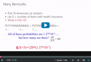
So now, what’s the probability that I
get 3 of these Americans with health insurance?
Well, I have to add up all of the possibilities with X=3.
So I have to add up the probability that
that happens, and
then I have to add that to the probability that this happens.
And then all the other ways that I have 3 yes’s and 7 no’s.
That’s gonna be the answer to my problem.
And all these probabilities are gonna be 1.37 times 10 to
the negative 7.
And the question is how many terms are there?
How many of these things do I have to add up?
Now that brings us to the question of how many ways
are there to rearrange 10 numbers?
This is the same question as the following.
So let’s suppose that there are 10 data scientists seated
in a row.
How many ways are there to pick a group of 3?
Now, there are how many ways to arrange them?
There are 10 ways to pick first data scientist.
And then once he’s chosen,
how many ways are there to pick the second data scientist, 9.
And then once that ones chosen, then there are eight left and
so on and so forth, so that’s ten factorial.
But then how many ways are there to arrange the 3 I picked?
Because it doesn’t matter in which order I pick those 3,
I just have to get 3 of them.
And, in fact, that, of course, is then 3 factorial, but
the same logic.
And then I don’t really care how the 7 that I didn’t pick
are arranged.
So how many ways to arrange them are there, it’s 7 factorial.
So we’re almost there, so the answer to this question then,
s 10 factorial divided by 3 factorial 7 factorial.
This is the number of ways to
rearrange all the data scientists.
This is the number of ways to rearrange the 3 that I pick,
cuz I don’t care what arrangement they’re in.
And then this is the number of ways to arrange the 7
that I don’t pick.
And the answer here is 120.
And more generally, the answer is n choose k.
This is the notation for n choose k.
n is the number of data scientists,
k is the number of them I’m gonna pick.
And so, this is the number of ways to choose k out of n.
With that, we now know how many terms there are in this sum.
Remember, we knew that each probability was 1.37,
times 10 to the negative 7th, and
we didn’t know how many terms there were.
And the answer is, actually, 10 factorial divided by
3 factorial 7 factorial, which is 120.
It’s the number of ways to pick
3 Americans out of 10.
So the answer to the problem,
this problem over here looks like that.
It’s 120 terms times each term which is 1.37
time 10 to the negative 7.
Let us take a deep breath and
review the process by which we got to that answer.
So, let us go over the problem first.
So, we want to pick 10 Americans at random,
X is gonna be the number of them that have health insurance.
And I want to know what the probability is, that X is 3.
And other words, what’s the probability that of the 10
Americans I pick, 3 of them have health insurance.
We’ve already solve the problem, so I wanna go backward through
the calculation that we made to get to that answer.
So we decided that the answer was 120 times 1.37
times 10 to the negative 7.
Now this number here, 1.37 times 10 to the negative 7,
we got that thing by probability 0.89 to have health
insurance, and 3 Americans out of our 10 have it.
And then 0.11 is the probability not to have health insurance in
7 Americans in our 10 are gonna have that.
And then 120 we got from this calculation over here
which is the number of ways I can pick 3 out of 10.
And that ended up being the answer.
And then if I multiply it all out I get this number over here
which is the final one.
What I wanna do now is write
this in more general notation to solve a more general problem.
And that’s the formula that I want to show you.
This is actually the punchline, this is the formula for
the binomial distribution.
Now I’m gonna discuss it more in the next slide.
But I want you to see that it looks just like
what we computed already.
So pick n Americans at random, before n was 10,
but now it’s general.
Each American has probability p of having health insurance,
the p before was 0.89.
And then my random variable is the number of them
with health insurance.
I want to know, I wanna formula of the probability that
that random variable equals a particular value, little x.
So here is the formula, right here.
So this thing is the number of ways I can choose
x objects out of n total.
And then p is the probability of success for
each of the Bernoulli trials, each of the n Bernoulli trials.
And we’re gonna have x successes and n-x failures.
And so this is exactly what we just computed in the example.
So this is the binomial distribution.
You have n independent trials,
each one has the same probability of success.
And the probability of x successes out of n,
little x successes out of n,
is exactly this formula, this is the binomial distribution.
Now, you got through that, that was the hard part.
I will tell you some interesting facts about the binomial
distribution that you might wanna keep in your head.
So here they are, the mean of the binomial distribution, or
the expectation of the binomial distribution is n times p.
So you have n independent trials each with
the probability of success p, the mean is n times p.
And then the spread of that distribution,
the spread of the binomial, the variance of it is np(1- p).
Okay so these are two facts that I keep in my head.
And I carry them with me all the time because I end up using them
fairly often.
And now you understand the binomial distribution.
End of transcript. Skip to the start.

Data Science Essentials & Machine Learning

Curriculum

Probability and Random Variables – Discrete Probability Distributions

Discrete Probability Distributions

Downloads and transcripts

Video

Transcripts

Modal title