- Home
- Courses
- Data Science
- Data Science Essentials & Machine Learning
Curriculum
- 8 Sections
- 69 Lessons
- 4 Weeks
Expand all sectionsCollapse all sections
- Before You StartIntroduction4
- Module 1: Introduction to Data Science12
- 3.1Principles of Data Science – Data Analytic Thinking
- 3.2Principles of Data Science – The Data Science Process
- 3.3Further Reading
- 3.4Data Science Technologies – Introduction to Data Science Technologies
- 3.5Data Science Technologies – An Overview of Data Science Technologies
- 3.6Data Science Technologies – Azure Machine Learning Learning Studio
- 3.7Data Science Technologies – Using Code in Azure ML
- 3.8Data Science Technologies – Jupyter Notebooks
- 3.9Data Science Technologies – Creating a Machine Learning Model
- 3.10Data Science Technologies – Further Reading
- 3.11Lab Instructions
- 3.12Lab Verification
- Module 2: Probability & Statistics for Data Science21
- 4.1Probability and Random Variables – Overview of Probability and Random Variables
- 4.2Probability and Random Variables – Introduction to Probability
- 4.3Probability and Random Variables – Discrete Random Variables
- 4.4Probability and Random Variables – Discrete Probability Distributions
- 4.5Probability and Random Variables – Binomial Distribution Examples
- 4.6Probability and Random Variables – Poisson Distributions
- 4.7Probability and Random Variables – Continuous Probability Distributions
- 4.8Probability and Random Variables – Cumulative Distribution Functions
- 4.9Probability and Random Variables – Central Limit Theorem
- 4.10Probability & Random Variables – Further Reading
- 4.11Introduction to Statistics – Overview of Statistics
- 4.12Introduction to Statistics – Descriptive Statistics
- 4.13Introduction to Statistics – Summary Statistics
- 4.14Introduction to Statistics – Demo: Viewing Summary Statistics
- 4.15Introduction to Statistics – Z-Scores
- 4.16Introduction to Statistics – Correlation
- 4.17Introduction to Statistics – Demo: Viewing Correlation
- 4.18Introduction to Statistics – Simpson’s Paradox
- 4.19Introduction to Statistics – Further Reading
- 4.20Introduction to Statistics – Lab Instructions
- 4.21Introduction to Statistics – Lab Verification
- Module 3: Simulation & Hypothesis Testing16
- 5.1Simulation – Introduction to Simulation
- 5.2Simulation – Start
- 5.3Lab
- 5.4Simulation – Demo: Performing a Simulation
- 5.5Simulation – Further Reading
- 5.6Hypothesis Testing – Overview
- 5.7Hypothesis Testing – Introduction
- 5.8Hypothesis Testing – Z-Tests, T-Tests, and Other Tests
- 5.9Hypothesis Testing – Test Examples
- 5.10Hypothesis Testing – Type 1 and Type 2 Errors
- 5.11Hypothesis Testing – Confidence Intervals
- 5.12Hypothesis Testing – Demo with R & Python
- 5.13Hypothesis Testing – Misconceptions
- 5.14Hypothesis Testing – Further Reading
- 5.15Hypothesis Testing – Lab Instructions
- 5.16Hypothesis Testing – Lab Verification
- Module 4: Exploring & Visualizing Data4
- Module 5: Data Cleansing & Manipulation4
- Module 6: Introduction to Machine Learning4
- Final Exam & Survey4
Probability and Random Variables – Cumulative Distribution Functions
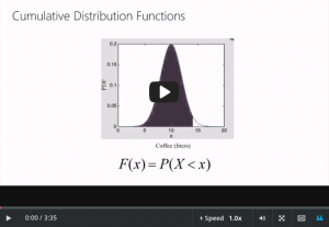
Cumulative Distribution Functions
Downloads and transcripts
Video transcript
- Start of transcript. Skip to the end.
- Now the CDF tells you the probability for
- random variable x to be below a certain value.
- So in our case over here, it’s 14.
- Okay, so this area under here, that’s the probability that
- the random variable’s less than or equal to 14.
- And the CDF function is written just like this.
- F(14), that’s the probability of the random variable to take
- on a value below 14.
- And I can write it more generally, so
- if I can write it for a general x.
- So for any of amount of coffee x that Steve might drink,
- the CDF gives the probability to drink less than that value.
- Now, does it matter whether I write less than or
- equal to here or just less than?
- And the answer is no, it doesn’t matter,
- because the probability that he’ll drink
- exactly that value x down to the molecule is 0.
- For continuous distributions, doesn’t matter whether this is
- strict equality or less than or equal to.
- So this subtraction that we were doing earlier,
- this can actually be written in terms of the CDFs.
- So if we want the probability that X is between 10 and 14,
- it’s the CDF at 14 minus the CDF at 10.
- And I can write it like this.
- And if I want the probability that Steve is gonna drink more
- than a certain value, like 11 liters, then I can actually
- get that by remembering that the area under the whole thing
- is 1 and subtracting the area to the left of 11 here.
- Okay, so what is the smallest possible value for the CDF?
- And at 0 all the way on the left, okay?
- So if X is -10, that’s way over here, then F is about 0.
- Now what about 0.25, okay?
- So if X is 8, then the area under here is about 0.25.
- This is about a quarter of the area under the whole thing.
- That’s a quarter probability to get less than 8.
- Then what about 10?
- F(10) is about 0.5,
- because that’s really where the center of the distribution is.
- F(12) is about 0.75 and then F(20) is about 1,
- so if I actually plot out what F looks like, it looks like this.
- So it’s 0 all the way to the left, and
- then when I get to about 8, it’s 0.25.
- When I get to 10 it’s about 0.5, I get up to 12 it’s about 0.75,
- and when I get up to 20, it’s 1, okay.
- So now you
- see I seem to be drawing bumps very often as my example of what
- a PDF ought to look like, which means the CDF
- always ends up looking kinda like that function down here.
- Now, there is a very good reason that I keep drawing bell curves
- like this and I will tell you what it is.
- It is called the central limit theorem and that is up next.
- End of transcript. Skip to the start.