- Home
- Courses
- Data Science
- Data Science Essentials & Machine Learning
Curriculum
- 8 Sections
- 69 Lessons
- 4 Weeks
Expand all sectionsCollapse all sections
- Before You StartIntroduction4
- Module 1: Introduction to Data Science12
- 3.1Principles of Data Science – Data Analytic Thinking
- 3.2Principles of Data Science – The Data Science Process
- 3.3Further Reading
- 3.4Data Science Technologies – Introduction to Data Science Technologies
- 3.5Data Science Technologies – An Overview of Data Science Technologies
- 3.6Data Science Technologies – Azure Machine Learning Learning Studio
- 3.7Data Science Technologies – Using Code in Azure ML
- 3.8Data Science Technologies – Jupyter Notebooks
- 3.9Data Science Technologies – Creating a Machine Learning Model
- 3.10Data Science Technologies – Further Reading
- 3.11Lab Instructions
- 3.12Lab Verification
- Module 2: Probability & Statistics for Data Science21
- 4.1Probability and Random Variables – Overview of Probability and Random Variables
- 4.2Probability and Random Variables – Introduction to Probability
- 4.3Probability and Random Variables – Discrete Random Variables
- 4.4Probability and Random Variables – Discrete Probability Distributions
- 4.5Probability and Random Variables – Binomial Distribution Examples
- 4.6Probability and Random Variables – Poisson Distributions
- 4.7Probability and Random Variables – Continuous Probability Distributions
- 4.8Probability and Random Variables – Cumulative Distribution Functions
- 4.9Probability and Random Variables – Central Limit Theorem
- 4.10Probability & Random Variables – Further Reading
- 4.11Introduction to Statistics – Overview of Statistics
- 4.12Introduction to Statistics – Descriptive Statistics
- 4.13Introduction to Statistics – Summary Statistics
- 4.14Introduction to Statistics – Demo: Viewing Summary Statistics
- 4.15Introduction to Statistics – Z-Scores
- 4.16Introduction to Statistics – Correlation
- 4.17Introduction to Statistics – Demo: Viewing Correlation
- 4.18Introduction to Statistics – Simpson’s Paradox
- 4.19Introduction to Statistics – Further Reading
- 4.20Introduction to Statistics – Lab Instructions
- 4.21Introduction to Statistics – Lab Verification
- Module 3: Simulation & Hypothesis Testing16
- 5.1Simulation – Introduction to Simulation
- 5.2Simulation – Start
- 5.3Lab
- 5.4Simulation – Demo: Performing a Simulation
- 5.5Simulation – Further Reading
- 5.6Hypothesis Testing – Overview
- 5.7Hypothesis Testing – Introduction
- 5.8Hypothesis Testing – Z-Tests, T-Tests, and Other Tests
- 5.9Hypothesis Testing – Test Examples
- 5.10Hypothesis Testing – Type 1 and Type 2 Errors
- 5.11Hypothesis Testing – Confidence Intervals
- 5.12Hypothesis Testing – Demo with R & Python
- 5.13Hypothesis Testing – Misconceptions
- 5.14Hypothesis Testing – Further Reading
- 5.15Hypothesis Testing – Lab Instructions
- 5.16Hypothesis Testing – Lab Verification
- Module 4: Exploring & Visualizing Data4
- Module 5: Data Cleansing & Manipulation4
- Module 6: Introduction to Machine Learning4
- Final Exam & Survey4
Probability and Random Variables – Continuous Probability Distributions
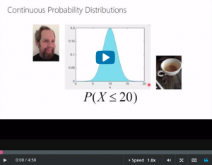
Continuous Probability Distributions
Downloads and transcripts
Video Transcript
- Start of transcript. Skip to the end.
- Okay, so let’s talk about continuous probability
- distributions and continuous random variables.
- Now if I wanted to write a table that
- would tell me for each outcome what the probability is for
- a continuous random variable, this would not work.
- This would fail very, very badly.
- There are uncountably infinite amount of values in this table
- and all the probabilities are exactly zero.
- So that does not work.
- But I can draw a curve that represents something
- meaningful for continuous random variables,
- which is the probability distribution function.
- There’s Steve, y’all know him, and this is a distribution.
- And so the higher this curve is, the more likely the value is.
- So this particular distribution is the distribution of how much
- coffee Steve Elston is going to consume in liters over the next
- week.
- Okay, so he’s more likely to consume somewhere around ten
- liters than he is to consume somewhere around zero liters.
- But the probability that he’ll consume any
- particular exact amount of coffee is exactly zero.
- Right, so it no longer make sense to say something like
- the probability he’ll consume 8.23576 liters of coffee is 0.1,
- all right, that makes no sense here.
- The probability is zero.
- It makes much more sense to say what is the probability
- that Steve will consume between 10 and 15 liters?
- And that is going to be this much.
- The shaded area here is the area under this curve, okay?
- That’s the probability, to get between these two values.
- So if I try to ask what the probability is to land on a
- particular value, the area under that single value will be zero.
- And if I look at a range of values it won’t be zero.
- Or you could say what’s the probability
- that Steve will have less than ten liters?
- And that’s about a 50% probability or 0.5.
- And now you could say,
- what’s the probability that he’ll have less than 20 liters?
- Looks like he pretty much always has less than 20 liters.
- That’s a good thing,
- because it’s probably not good to drink quite that much coffee.
- So this probability is about one.
- Okay, that’s the largest probability you can ever get.
- Right, one is the total area under this whole thing.
- So this thing integrates to one and
- the areas under it are probabilities.
- Those are the key aspects of the probability density function.
- Now these PDFs come in all shapes and
- sizes, it doesn’t have to look like a bump.
- It can look like two bumps or it can look very flat, or
- it can, whatever.
- It just has to integrate to one.
- So this is the probability density function for
- what’s called the uniform distribution.
- It’s completely flat.
- So this uniform distribution means that any value between,
- any value between 10 and 20 is sort of equally probable, okay?
- So, but remember it doesn’t make sense to talk about
- a particular value.
- But what I can say is that the probability to get between
- 10 and 12 is that area there.
- And you can probably figure out what that area is if the whole
- thing has to integrate to 1 and that’s 10 and that’s 20,
- then the area is 0.2, okay.
- So 2 wide by one-tenth high, so, 0.2.
- So back to this.
- How do I calculate these things?
- Well, the way we usually do
- it is we do it by subtracting two quantities.
- So we’d calculate this quantity over here, and
- then I would subtract this one, to get the probability I want,
- which is the thing in pink.
- So now the question of computing probabilities becomes a question
- of computing the areas to the left of things,
- to the left of any particular outcome.
- And this brings me to the discussion of cumulative
- distribution functions or CDFs.
- End of transcript. Skip to the start.