Probability and Random Variables – Central Limit Theorem

Video transcript

1. Start of transcript. Skip to the end.
2. Well, let me tell you about the central limit theorem and
3. the normal distribution.
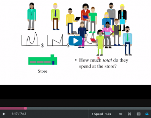
4. Now, everyday a bunch of customers go into a store,
5. each with their own kooky distribution
6. of how much they wanna spend.
7. Like, this guy wants to spend, sometimes a little bit,
8. sometimes a lot, but not much in between.
9. This person spends a little bit, a medium amount, or
10. a lot, sometimes an awful lot.
11. And this guy, he just likes ties.
12. So he always buys ties and there’s always this price.
13. Somewhere in this price range.
14. Now, the question is, at the end of the day,
15. the store counts the total amount of money that
16. they collect from all of these customers.
17. So how much total do they spend at the store?
18. And let’s assume we have a lot of customers in the store.
19. And we even have some students taking this course going
20. to the store, and bringing their computers to the store just for
21. fun, while they’re learning data science.
22. And each of them has their own distribution
23. of how much they spend.
24. Every evening, the store counts their total profit, and every
25. day it was slightly different than it was the day before.
26. And now we ask the store to
27. plot the distribution of it’s profits.
28. Here’s what it looks like.
29. A bump.
30. And we ask them what the center of the bump is, and magically as
31. it turns out, the center of this distribution of total profits
32. is exactly the sum of the means of the individual customers.
33. My goodness, that is cool.
34. Now, start over again.
35. Now, this is a totally different store with totally different
36. customers.
37. In fact, it’s on the other side of the world.
38. Everything’s totally different.
39. And now we ask,
40. what is the distribution of this store’s profits?
41. And rather interestingly, ha, ha,
42. they also end up with a very similar looking sort of bump.
43. Totally different store.
44. Totally different customers, and
45. yet, a single bump with the same shape.
46. And the mean has the same formula too.
47. It’s the sum of the means of the customers’ individual means.
48. But what the heck is going on here?
49. Are these stores in cahoots?
50. Did they to each other and
51. negotiate the distribution of their sales?
52. No way.
53. It turns out, and get this, it always happens.
54. The same bump with the same shape, right?
55. It might be stretched out a bit, or it might be squeezed a bit,
56. or scaled a bit, or
57. shifted a bit, but it’s really the same shape.
58. So this is called the normal distribution.
59. And its shape is given by this particular formula, and
60. it’s always the same formula.
61. It’s always the same shape.
62. And the formula has a mean in it, mu, the mean of this thing.
63. And the standard deviation sigma,
64. that’s the measure of the spread of that distribution.
65. Now if you know those two things, if you know the mean and
66. you know the sigma, you have the whole formula.
67. So you know the whole shape of that curve.
68. And it alway integrates to one.
69. Now funny things happen when you fiddle with the mean and
70. the variance there.
71. So you can get these very kinda peaky normal distributions
72. with small standard deviations.
73. Or you could get these very broad ones with large standard
74. deviations.
75. And the mean can actually be any value it wants to be.
76. And the standard deviation, as long as it’s positive,
77. can be anything.
78. And there’s that formula again.
79. So, as long as you know the mean and the standard deviation,
80. you got the full shape.
81. Now, the cool thing is this fact that I told you,
82. that the sum of a large number of independent random variables
83. is approximately normal.
84. And this is actually called the central limit theorem.
85. And this is one of the most famous theorems in the world,
86. the central limit theorem.
87. So, even though all of the different customers had
88. a totally different distribution,
89. when you add them up, the sum is approximately normal.
90. So let’s have X1 through Xn be independent random variables.
91. Their means are mu 1 through mu n.
92. The standard deviations are sigma 1 through sigma n.
93. Now I take their sum.
94. Okay, this is the total sales for the store.
95. And the Xs are the sales for the individual customers.
96. And now as it turns out, that sum is approximately
97. normal with mean, which is the sum of the means.
98. So the mean of the sum is the sum of the means.
99. And the variance of the sum turns out to be
100. the sum of the variances of the independent random variables.
101. Of course, the standard deviation is just the square
102. root of the variance.
103. Now, this theorem only works when
104. the variables are independent.
105. So you just have to make sure that that’s true.
106. And that’s true for
107. sales because each customer comes into the store and
108. doesn’t worry about what another customer is doing.
109. Now the larger n is, the closer to normal,
110. that s, that sum is.
111. And it turns out that if the Xn’s are actually normal in
112. the first place, then their sum is normal anyway.
113. Exactly normal.
114. So if you start out with weird distributions though,
115. then n needs to be a bit larger to look normal.
116. Now, because of the central limit theorem,
117. this distribution and this formula pops up all the time.
118. Now, this formula is not something that a person made up,
119. it’s some thing that exists in nature.
120. It’s just as natural as the patterns you might find when
121. looking at water waves or seashells.
122. It’s something that comes with the earth.
123. It’s the distribution of the amount of rain in
124. Boston over the year.
125. It’s the distribution of test grades
126. assuming no systematic cheating.
127. And it’s the distribution of anything that’s a sum of
128. independent events.
129. This is like equals mc squared for probability.
130. You might say, well, but I already
131. thought you told us about sums of independent random variables?
132. Doesn’t the binomial distribution come from a sum of
133. independent random variables?
134. Well, as it turns out, the limiting binomial distribution
135. is actually normal, so isn’t that lovely?
136. So, if I start out with just one trial with probability 0.5,
137. the binomial distribution is pretty boring,
138. it just looks like this, right?
139. This is just a fair coin with a single coin flip.
140. Half the time you’ll get 0, half the time you’ll get 1.
141. Then when I start flipping more coins
142. it starts to look a little bit more normal.
143. Flip 3 coins.
144. 4 coins.
145. 5, and then we can flip 10 coins, 100 coins, and
146. 1000 coins.
147. And then you’ll see what looks like very much a beautiful
148. normal looking distribution.
149. So the limiting binomial is a normal.
150. Isn’t that lovely?
151. Okay, so, yes, so that’s the point.
152. For large n, the binomial distribution actually becomes
153. the normal distribution.
154. End of transcript. Skip to the start.