Introduction to Statistics – Z-Scores

Video transcript

1. Start of transcript. Skip to the end.
2. So this lecture is all about how to view data with respect to
3. other data.
4. So if you’re telling me that you’re an excellent salesman
5. because you sold $100,000 worth of widgets,
6. I have no idea what that means.
7. You can be terrible compared to your peers, but
8. how would I know that based on what you told me?
9. If you tell me the z-score or what percentile you were,
10. then that’s a different story, right, that’s meaningful.
11. Obviously, variance in correlation are about
12. the relationships between two random variables.
13. Let’s start.
14. It’s helpful to think of values relative to other values within
15. the same distribution, and
16. that’s what a z-score tells you, it tells you where a point is
17. relative to other points in the distribution.
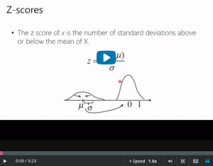
18. It’s the number of standard deviations above or
19. below the mean for a particular point.
20. It’s helpful to think of values relative to other values within
21. the same distribution.
22. If I tell you that I just sold 1200 units,
23. that doesn’t mean much, cuz you have no idea how good of
24. a salesman I am, because you don’t have enough context.
25. What if I told you the mean was a 1000 units?
26. Still, that doesn’t tell you very much.
27. You have no idea how unusual it is to go above 1200 units.
28. Is that very unusual?
29. Or it was just I was slightly above the mean?
30. What you need also is the standard deviation.
31. If I tell you it is 100 units, then you know I’m in business
32. because I’m selling two standard deviations above the mean.
33. Now, here’s say a histogram here and
34. I’m selling here at 1200 and the mean is over here.
35. Now the vast majority of other salespeople sell much
36. less than 1200, so I’m at the top of the pile if I’m up here.
37. Of course, this assumes that salesmen have an approximately
38. normal distribution, which may or may not be true for
39. a specific company, but we’ll let that go for now.
40. The z score of a point x is the number of standard deviations
41. above or below the mean of X.
42. And an easy way to compute that is to use this formula
43. right here.
44. But that looks a little complicated, so
45. let’s break it down a bit.
46. Well, let us start with the original PDF of X.
47. Let’s say that this is X’s PDF, X is random variable.
48. Then I’m gonna subtract the mean, so now this
49. thing has mean 0 because I subtracted the mean, what I did.
50. When I divide by the standard deviation here,
51. I actually squish the distribution, so
52. the distribution now has mean 0 and standard deviation 1.
53. When I think about one standard deviation above the mean of X,
54. it’s exactly at the point 1 of this new distribution where
55. z is 1.
56. What I did when I subtracted the mean and divided by the standard
57. deviation is that I shifted the distribution to have mean 0 and
58. I scaled it to have standard deviation 1,
59. where I standardized the distribution.
60. In this way, z measures how many standard deviations X is
61. above or below the mean.
62. Now if you’re working with data, you don’t actually have
63. the mean mu, you only have the sample mean X bar.
64. People often get confused and call these z-scores, in fact,
65. I do it myself but they’re actually really sample z-scores.
66. The sample z-score of X is actually the number of sample
67. standard deviations above or below the sample mean.
68. Okay, so here is a histogram of my data, and
69. you can see that the sample mean is 1000.
70. And my sample z-score is about 2 because
71. I’m 2 sample standard deviations above the sample mean.
72. Just to give you some perspective, let me discuss for
73. you how rare that actually is.
74. Here is a standard normal with mean 0 and variance 1.
75. Now it turns out that 68% of the time,
76. you’re within one standard deviation of the mean.
77. Now you can’t calculate this analytically, by the way,
78. you actually need a computer to do this to get that 68%.
79. As it turns out that 95% of the time,
80. you’re within two standard deviations of the mean.
81. And 99.7% of the time,
82. you’re within three standard deviations of the mean.
83. Now you can put it into context.
84. Though I sold 1200 units, the mean is 1000 and
85. the standard deviation is 100, but the z-score is 2.
86. So I sold two standard deviations above the mean and
87. the probability to be that extreme is actually only 2.5%.
88. So I’m a pretty unusual sales person.
89. End of transcript. Skip to the start.