- Home
- Courses
- Data Science
- Data Science Essentials & Machine Learning
Curriculum
- 8 Sections
- 69 Lessons
- 4 Weeks
Expand all sectionsCollapse all sections
- Before You StartIntroduction4
- Module 1: Introduction to Data Science12
- 3.1Principles of Data Science – Data Analytic Thinking
- 3.2Principles of Data Science – The Data Science Process
- 3.3Further Reading
- 3.4Data Science Technologies – Introduction to Data Science Technologies
- 3.5Data Science Technologies – An Overview of Data Science Technologies
- 3.6Data Science Technologies – Azure Machine Learning Learning Studio
- 3.7Data Science Technologies – Using Code in Azure ML
- 3.8Data Science Technologies – Jupyter Notebooks
- 3.9Data Science Technologies – Creating a Machine Learning Model
- 3.10Data Science Technologies – Further Reading
- 3.11Lab Instructions
- 3.12Lab Verification
- Module 2: Probability & Statistics for Data Science21
- 4.1Probability and Random Variables – Overview of Probability and Random Variables
- 4.2Probability and Random Variables – Introduction to Probability
- 4.3Probability and Random Variables – Discrete Random Variables
- 4.4Probability and Random Variables – Discrete Probability Distributions
- 4.5Probability and Random Variables – Binomial Distribution Examples
- 4.6Probability and Random Variables – Poisson Distributions
- 4.7Probability and Random Variables – Continuous Probability Distributions
- 4.8Probability and Random Variables – Cumulative Distribution Functions
- 4.9Probability and Random Variables – Central Limit Theorem
- 4.10Probability & Random Variables – Further Reading
- 4.11Introduction to Statistics – Overview of Statistics
- 4.12Introduction to Statistics – Descriptive Statistics
- 4.13Introduction to Statistics – Summary Statistics
- 4.14Introduction to Statistics – Demo: Viewing Summary Statistics
- 4.15Introduction to Statistics – Z-Scores
- 4.16Introduction to Statistics – Correlation
- 4.17Introduction to Statistics – Demo: Viewing Correlation
- 4.18Introduction to Statistics – Simpson’s Paradox
- 4.19Introduction to Statistics – Further Reading
- 4.20Introduction to Statistics – Lab Instructions
- 4.21Introduction to Statistics – Lab Verification
- Module 3: Simulation & Hypothesis Testing16
- 5.1Simulation – Introduction to Simulation
- 5.2Simulation – Start
- 5.3Lab
- 5.4Simulation – Demo: Performing a Simulation
- 5.5Simulation – Further Reading
- 5.6Hypothesis Testing – Overview
- 5.7Hypothesis Testing – Introduction
- 5.8Hypothesis Testing – Z-Tests, T-Tests, and Other Tests
- 5.9Hypothesis Testing – Test Examples
- 5.10Hypothesis Testing – Type 1 and Type 2 Errors
- 5.11Hypothesis Testing – Confidence Intervals
- 5.12Hypothesis Testing – Demo with R & Python
- 5.13Hypothesis Testing – Misconceptions
- 5.14Hypothesis Testing – Further Reading
- 5.15Hypothesis Testing – Lab Instructions
- 5.16Hypothesis Testing – Lab Verification
- Module 4: Exploring & Visualizing Data4
- Module 5: Data Cleansing & Manipulation4
- Module 6: Introduction to Machine Learning4
- Final Exam & Survey4
Introduction to Statistics – Correlation
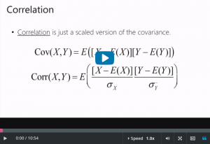
Correlation
Downloads and transcripts
Video transcript
- Start of transcript. Skip to the end.
- Let’s talk about covariance and correlation.
- There’s a company that rents bikes and scooters to commuters.
- And people get to choose either a bike or a scooter,
- whichever they want.
- And as it turns out, there’s a negative correlation between
- the number of bike customers and the number of scooter customers.
- So what does that actually mean?
- So you can see a negative correlation in the scatter plot
- clearly, but
- what is the technical definition of correlation?
- Well, let’s think about it this way.
- So this is the average number of scoot customers per day here,
- and here’s the average number of bike customers.
- So what it says is that if there are more than average scoot
- customers on a particular day, there are probably fewer
- than average bike customers and vice versa.
- Okay, so there that is.
- Higher than average scoot corresponds to lower than
- average bike, right, higher than average scoot and
- lower than average bike.
- Okay, so, vice versa, if Monster Scoot has fewer customers than
- their usual average, it probably means Monster Bike has higher
- than average number of customers that day.
- And so that brings me to a formal definition of
- covariance and correlation.
- Let’s start with covariance.
- Okay, so let’s say whether X is above or below its mean.
- And I’m writing the mean here, the mean of X,
- as the expectation of X.
- And I used the notation mu before, but
- this means the same thing.
- And this notation is just as common as the mu notation.
- So we’re looking at whether X is above or below its mean.
- And now let’s see if Y is above or below its mean.
- So two random variables, X and Y,
- if X is higher than its mean when Y is lower than its mean,
- then this thing is gonna be negative.
- Actually let’s just go through all the combinations.
- So if X is higher than its mean and
- Y is higher than its mean, then this is positive.
- Now, if X is above its mean, and Y is below its mean, when you
- multiply them together, you get something that’s negative.
- And I filled in the rest.
- Now if X is below its mean when Y is below its mean,
- we’re gonna be multiplying two negative numbers together, and
- then we’ll get a positive one.
- Okay, so this is the definition of the covariance.
- It’s just the expectation of this quantity in here.
- So, now it’s all about how often things happen.
- If we’re often in a situation where X and Y vary together,
- then the product in here will often be positive,
- and then the expectation will be positive.
- Okay, so that’s for the population.
- What if you only have data?
- Then you need to compute the sample covariance which is
- this thing down here.
- It’s exactly the same thing as the covariance.
- The only difference is that you can compute it from your data
- which is 1 to n.
- And then again there’s this mysterious n-1 over there that
- you really should not pay attention to cuz it’s just
- an issue of bias.
- Like I said, it’s already in the software to compute that for
- you so you shouldn’t pay attention to it.
- Then what happens if you take the covariance of X with itself?
- So X, the Y is also equal to X.
- Look at this, does that look familiar?
- It should, because it is exactly the variance, and
- this is the same definition we had earlier.
- Take the distance of X from its mean,
- square it to get the squared distance from the mean, and
- take the expectation, and that’s the variance.
- And then this one here is the sample variance, again,
- with that silly n-1 over there.
- And the sample variance has a particular notation, and
- it is called s squared.
- Now the issue with covariance is that it’s not in units that make
- any sense.
- So correlation is a version of covariance, but where we scaled
- its value so that the largest possible correlation is one,
- and the smallest possible value is minus one.
- And so that’s what these terms are here.
- So this is the standard deviation of X, and
- this is the standard deviation of Y.
- And when you scale this quantity by these two terms, then
- the largest value is one and the smallest value is minus one.
- Okay, and here is the sample correlation.
- And again, you get that silly n-1 term.
- And then these become quantities that you can compute from your
- data, namely the sample standard deviations of X and of Y.
- Now since correlations are always between +1 and
- -1, a correlation of 0.7 say, that’s actually meaningful.
- I can really understand it on this scale between 1 and -1.
- Here’s a nice plot showing some of the data from the automobile
- pricing data set.
- Now each car in this data set gets a dot which represents its
- price, and then the size of the engine of the car.
- And you can definitely see that there’s
- a clear positive correlation there.
- As price goes up,
- you would definitely expect the engine size of a car to go up.
- If you paid more for the car, you’re paying for
- a bigger engine.
- And the increase pretty much follows a straight line here.
- And it follows the straight line well enough
- that the correlation is actually 0.89.
- See the covariance here, that’s in weird units, so it’s really
- hard to figure out what that number means intuitively.
- But the correlation,
- that’s actually much easier to deal with.
- And then here’s more of that same data set, so this is bore
- diameter which is the size of a part of the engine, and price.
- This bore diameter, it does correlate with price, but
- it’s not as closely correlated as the engine size.
- So here the correlation is 0.55, and again I have this mysterious
- covariance value that I don’t know exactly what to do with.
- Now this is city miles per gallon versus price,
- and here you can see a negative correlation.
- I guess that as price goes up the cars must not be as
- efficient, probably because they have bigger engines or
- something, I don’t know.
- Anyway, so the correlation is -0.7.
- And that again that’s meaningful because the lowest it can be is
- a -1.
- Now be careful because people widely confuse
- correlation with causation.
- Correlation is really, really not causation.
- And here is the quintessential example of why that’s not true.
- It turns out that health, human health,
- has a negative correlation with how wealthy you are.
- So you see points like this.
- If you plot sort of the individuals around the world,
- you’ll notice that the healthier they are, the less wealthy they
- are, and the more wealthy they are, the less healthy they are.
- So why in the world is that?
- And if you think for a minute, you’ll figure it out.
- And you’ll figure out that there is some piece of information I
- didn’t tell you, which is the age of these individuals.
- Because older people tend to be wealthier but less healthy, and
- younger people tend to be not as wealthy, but
- definitely more healthy.
- So what does that mean?
- This is not causal.
- It doesn’t mean that poor health causes you to be rich.
- And it also doesn’t mean that being rich causes you to be
- unhealthy.
- There’s nothing causal here.
- But there’s a correlation.
- I can predict health from wealth.
- I can predict wealth from health without anything causal in there
- at all.
- Now in machine learning, which we’ll get to,
- prediction is the name of the game.
- It’s not causality necessarily.
- There are some special branches of machine learning that
- are sort of concerned with causality.
- But for the most part,
- machine learning is just about predicting the future from data,
- not necessarily understanding the causal mechanisms.
- And so that’s a longer discussion that
- I really don’t wanna get into too much here.
- It’s just nice,
- though, that you don’t have to worry about causality because
- not having to worry about that makes things much
- easier from a practical perspective.
- You can just predict without worrying about the causes.
- So let’s say that you’re trying to predict whether someone will
- want a coupon for your store.
- But you don’t have to worry about why they will take that
- coupon or why they might want the product.
- All you have to do is use correlations to guess whether
- she might want the coupon.
- So for instance you could say, it’s Tuesday, and
- she often takes coupons on Tuesdays.
- So let’s enter a coupon.
- Who cares why she likes coupons on Tuesdays,
- we just know she does.
- Or we could say, people like her want this coupon,
- so let’s send it to her.
- Now machine learning is all about combining the right
- correlations to be able to predict accurately.
- But you can’t make conclusion about causality unless you learn
- more about causal inference techniques, which is really for
- another day.
- End of transcript. Skip to the start.