Hypothesis Testing – Demo with R & Python

Demo: Hypothesis Testing

To see how to perform a T-Test using R, watch the first video in this topic. For a Python-based demonstration, scroll down and watch the second video.

Hypothesis Testing with R

Downloads and transcripts

Video

Download video file

Transcripts

Hypothesis Testing with Python

Downloads and transcripts

Video

Download video file

Transcripts

Video Transcript – Hypothesis Testing with R

Start of transcript. Skip to the end.
Hi and welcome so Cynthia has been
talking about two concepts we use quite
often in statistics hypothesis testing
and confidence intervals and in this
demo I’m going to try to pull those two
concepts together to show you a
practical example and the example we’re
going to look at is comparing the
heights of adult children to the heights
of their parents and the data set we’re
going to use is actually of historical
significance in statistics Francis
Galton who invented the regression
method published his original paper and
1886 and these data were what Frank
gotten used to in that paper
we’re not going to look at the exact
problem Dalton looked at we’re going to
look at a different one which is
hypothesis testing on those data we can
load the data set
and then we’re going to just look at the
first few rows of that data set and just
talk about what is in these columns so
the first column is a case number that’s
just a sequential number that golden
gave these data family data and finally
number so gotten like these first four
children all come from the same family
family one and then there’s some
children from family to etc then we had
the height of their father and inches
the height of their mother and inches
the average height of the parents the
number of children in that family
a number assigned to each child their
gender whether they were male or female
and the height of that adult child
alright and let’s just look at the
dimensions of that data frame
and you can see the golden had 934 cases
where he went out in 19th century london
and actually measured these people in
these families
so
first off let’s make a histogram and
look at these data visually but we’re
going to look at a subset of these data
so in this line of code here I’m
subsetting the data so we’re only going
to have the sun’s basically the male
children
and then we’re going to make a histogram
of the height of those sons and
histogram of the height of their mothers
that’s what all this code is doing here
and there we have it so you can see the
child heights that’s the height of the
adult sons and the mothers height
obviously the height of the mother that
son and here’s the mean
of the mother site and the mean of the
sunlight they look quite different
there’s a fair amount of overlap between
those two distributions but the question
we need to look at is is that overlap
actually significant if we consider the
confidence intervals and perform a
hypothesis test on that
and we’re going to look at one other
case here so i’m going to subset this
date again so that we have
the gender now the child is female so
we’re going to compare the height of
daughters to the height of their mothers
let me run that code
and
have it so here’s the heights of the
daughters Instagram of heights the
daughters in the histogram of the
heights of their mothers and those means
are pretty close but again the question
is is that small different still
significant
so
down and a perform a t-test on this and
we’re going to look at the t-test we’re
going to look at the confidence interval
around that mean one of those means and
all this code does here so we’re doing
the two-sided t-test and let me just run
it
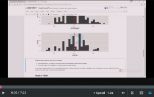
and there you have it so here’s this
first histogram is the heights of the
mothers with the mean height of the
mother and the mean height of the suns
and this dotted line here is the
confidence interval around the height of
the mother and you can see that that
difference between this height mean of
this site and the mean of that height is
quite different and it’s well outside
that ninety-five percent confidence
interval we can also look at the output
from this to set what’s called the
Walshes two-sample t-test and we get a
t-statistic that’s fairly large it’s got
a magnitude of about thirty
two-and-a-half pretty large degrees of
freedom that’s essentially a little less
than twice the number of mother-son
pairs our p-value is pretty tiny 10 to
the minus 16 is basically approaching 0
here and here’s the confidence interval
and that gonna be a little careful it’s
the confidence interval around the first
mean the mean of the mother so and
that’s how we got those Dottie lines
there
so one last thing to do here is we have
to look at testing this other
relationship which is between the mother
and the adult daughters see if those
Heights are significantly different
alright
so somewhat smaller degrees of freedom
there’s there’s fewer and the sample is
also the means are close together so now
the p-value is quite large in this case
points77 so it’s getting pretty close to
one RT statistic on the other hand is
extremely small it’s about point 3 so
and here’s our confidence interval and
notice that overlap 0 which is
interesting
and when we plot so that’s the
confidence interval the difference and
so here’s that confidence interval
plotted on the histogram upper and lower
and that mean of the daughters height is
pretty clearly within that ninety-five
percent confidence interval so what’s
the conclusion here so we have to accept
the null hypothesis in this case that
mothers and their adult daughters have
this the same height on average we can
reject that null hypothesis in this
first case where so we can reject the
null hypothesis that the height of the
Sun and the height of the mother are
effectively no different
so I hope that’s helped you understand
how we apply these concepts of the
confidence interval and the hypothesis
test to a data set where you’re actually
trying to compare whether two
populations have some significant
difference
End of transcript. Skip to the start.

Video Transcript -Hypothesis Testing with Python

Start of transcript. Skip to the end.
Hi and welcome so Cynthia has been
discussing two important concepts and
statistics which is confidence intervals
and hypothesis testing and in this demo
I’m going to use some tools from Python
to pull those two concepts together so
you can see how statisticians we
actually use those concepts to determine
whether say two populations are the same
or not and i’m going to use a very
famous data set
Francis Galton who invented regression
published this a paper on this data set
in 1886 it had to do with the heights of
parents and their adult children in 19th
century London he was using this to
introduce the whole concept of
regression at the time we’re going to do
something slightly different we’re going
to look at some hypothesis test we can
use with this very famous data set of
Dalton’s
so on my screen here i have this
notebook and i’m just going to run the
first sale here which just loads the
data
and we’ll look at the
first few rows of the data so what do we
have here we have the case which is just
a number galten gave it the family so
these people came from unique families
so golden gave them unique family
numbers the height of the father of the
family and inches the height of the
mother and family and inches the average
height of the parents the number of
children that that family had and then
the child number the gender of the child
and the height of that adult child
ok
and let’s have a look at the size of
that data set
you see there were 934 cases that were
golden apparently went out sometime in
the early eighteen eighties and measured
these people so to get a better feel for
that data set i’m going to create some
histograms and I’m going to do it for a
case here we’re going to look at the
gender which is the gender of the child
is male
so we’re going to compare and we’re
going to call that new data frame sons
and
we’re gonna make a histogram of sons
we’re going to compare the child height
which is the height of the Sun to the
height of his mother
so here we go
and oh and i put
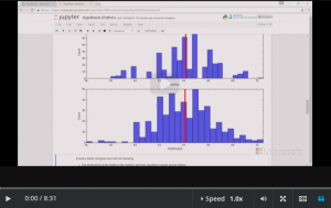
line at the mean so you can see here’s
the heights of the mothers
and the heights of the sons
and there’s quite a difference there’s
quite a bit of overlap in these
distributions as you can see but the
means are quite distinct and the
question is if we look at the confidence
intervals and perform a hypothesis test
on this data are these two populations
the height of the mothers and the
heights of there’s adult sons actually
different at some significance level
ok we’re going to get a different case
here which is we’re going to call this
daughter so it’s the same idea except
this time we’re going to look at we’re
going to compare the daughters the
height of the adult daughters to the
height of their adult i’m sorry the
height of the adult daughters to the
height of their mothers
and as you can imagine those
distributions look a lot more similar
there’s a lot more overlap in the
daughters and the means are virtually
the same but again is that
small difference significant at some
confidence interval or not your
confidence level or not so to resolve
that we’re going to use the t-test we’re
going to use the t-test at the five
percent or 0.5 confidence level and so
we’re going to and we’re going to do a
two-sided t-test here and we’ll print
out some other statistics like the
degrees of freedom the difference of the
means the t-statistic itself the p value
and the confidence interval and they
were going to plot those we’re going to
make histograms but we’re going to show
the confidence interval on those
histograms and that’s what all this code
is about so first we’ll do this between
between the sun’s the height of the
adult sons and the height of their
mothers
so let me run that for you
ok so first let’s look at the statistics
so we had you know there’s a large
number of degrees of freedom here over
900 because we had about 400 + + 20 or
440 pairs of
mothers and sons
the difference is about
five inches you can see there’s the
difference in the means they’re the t
statistic is fairly large it’s 39 and a
half
the p-value is quite small and
effectively at zero if you look at
something that’s 10 to the minus a
hundred and fifty-three but that’s just
a minute
computational anomaly it’s it’s
effectively a p a very low p value and
we can see the upper and lower
confidence interval around
basically the height of the mother so
we’re comparing the mother to the child
here so you need to sort of pay
attention to which cut which the
confidence interval around which of the
means you’re talking about and so
graphically we can see there’s quite a
difference here here’s our child height
so this is the height of the adult sons
cystogram here’s the histogram of the
height of the mothers and in those
dotted lines around the mean that’s the
confidence and that’s our ninety-five
percent confidence interval so this mean
is way outside that confidence interval
is just no doubt about it so yes we can
say based on all this
that Suns are significantly different in
height and their mothers but we can do
the same thing with that mothers
comparing the mothers to their daughters
so let me run that for you
and we get slightly fewer degrees of
freedom um because the means are so
close and in its
the difference is also only point 044
4.45 very small difference our
t-statistic now is less than one its
point 35 and our p-value is almost won
its points73 so it’s getting very close
to one and our confidence interval
overlap 0 so right there for that
difference that should tell us something
that’s that’s a bit odd
so if we plot those histograms again we
see the means for the adult daughters
and the mothers and the confidence
interval and clearly that mean is well
within that ninety-five percent
confidence interval so we need to reject
sorry we need to accept that null
hypothesis that
from the
others are the same as the heights of
the mother’s own dear i said something
wrong here
oh no that’s right i guess we can cut
that last bit out but that but that’s ok
so let me let me just do a wrap-up
so I hope this demo gave you some idea
of how in practice we use the concepts
of confidence intervals and hypothesis
test specifically in this case the t
test to determine if
two samples have significantly different
means
End of transcript. Skip to the start.

Data Science Essentials & Machine Learning

Curriculum

Hypothesis Testing – Demo with R & Python

Demo: Hypothesis Testing

Hypothesis Testing with R

Downloads and transcripts

Video

Transcripts

Hypothesis Testing with Python

Downloads and transcripts

Video

Transcripts

Modal title