Hypothesis Testing – Confidence Intervals

Confidence Intervals

Downloads and transcripts

Video

Download video file

Transcripts

Video Transcript

Start of transcript. Skip to the end.
So let’s talk about confidence intervals.
Let’s say we’re trying to figure out what is the average amount
of coffee in a mug?
Now the coffee machine can’t pour exactly the same amount of
coffee each time.
So there’s some distribution of how much coffee goes into a mug.
And I think it’s fair to
guess that the distribution is approximately normal.
Maybe that’s not fair, I’m not sure,
but it seems that a cup of coffee is a sum of lots of
independent little drops of coffee.
So the central limit theorem might kick in and
say that the total amount of coffee is approximately normal.
So if you buy that,
then the amount of coffee in a mug is normally distributed.
So, Steve Elston helps me out by drinking 100 cups of coffee and
I wrote down exactly how much coffee was in each cup.
And now, if I take the average of these numbers,
how close is it to the population average?
So here’s the average of the 100 cups.
It’s called x bar because it’s the average of the sample.
And now, I’m not allowed to know the true distribution, right?
I don’t know that.
I never can see that.
But I know that it’s normal.
So it could be here,
this could be true distribution with its mean mu.
Or it could be here, or here, or here and
I’ll never know which one it is.
What I’d really like to know is how far away x bar is from
true mu, whatever it is,
that we’re hoping to find out the x bar is close to mu.
And what I’d would really like to do is be able to draw
an interval around x bar.
And be able to say with some degree of certainty that mu is
close to x bar, that mu is in here with high probability,
with probability 1- alpha.
Now, I can tell you exactly what that interval is, but
it has a bunch of symbols in it that you don’t know.
Let me explain all these symbols, and
then I’m going to get back to this picture.
It’s gonna be the same picture, except that next time I show you
this, you’ll understand what all of these symbols mean.
Okay, so let’s start with the standard normal,
the mean 0 and standard deviation 1.
And I’m gonna ask you some questions about this
distribution.
I want to know, if I draw a point from the distribution,
what is the probability that it will be more than 1
standard deviation above the mean?
Now, remember, probabilities are areas here.
Okay, so what do you think the answer is?
What do you think the probability is to get a value
that’s in here when I draw randomly?
And the answer turns out to be about 15.87%, okay?
There’s a 15.87% chance that you’d draw a value that’s more
than 1 standard deviation above the mean.
Unfortunately there is no formula that people can write
down to get you from this 1 to this 15%, right?
The problem is that there’s no analytical form for
the area under the normal distribution.
Now, remember, since probabilities are integrals, and
integrals are sometimes not able to be computed analytically.
And this is a case where we can’t compute the integral using
a formula.
And that’s okay, cuz we have a look up table on the computer.
Any software you use will have a command that gets
you between these two numbers.
So, if you know that this probability is 15%,
then the computer can tell you that this corresponds to 1
standard deviation above the mean.
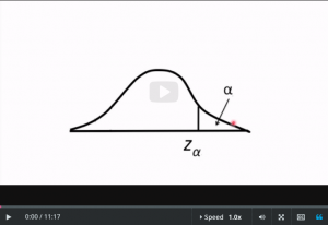
And it works for any alpha and
Z alpha and this is the usual notation.
Alpha’s the area, that is probability.
And Z offers the corresponding Z score.
Z alpha is the number of standard deviations above or
below the mean, so that this probability is alpha.
So if you give me Z alpha, whatever the heck it is.
Then there’s only one possible alpha corresponding to it, and
that’s in the computer’s look up table.
There’s a one to one correspondence which means if
you know alpha, you know Z alpha, and vice versa.
For any alpha you give me, I can give you Z alpha.
For any Z alpha you give me, I can give you alpha.
Okay, so I hope you get the point.
If you have the Z score,
you have the probability to be above it.
And now there’s this cool little trick that people use for
notation.
So you see the standard normal has mean 0.
So if you know alpha and Z alpha,
you automatically know the answer to this one.
If that’s alpha, what is the Z that corresponds to this?
And because the standard normal is symmetric,
the answer is actually -Z alpha.
Sometimes people like to ask questions about whether
something is unusual.
Meaning it could be in
one tail of the distribution or the other.
In that case they usually say that things
are okay 1-a of the time.
And then the probability of being unusual is alpha,
and that probability gets split between the two tails.
So again, you’re this many standard deviations
above the mean with probability, alpha/2.
Okay, so I think we’re ready to go back to confidence intervals.
You wanna know
what’s the average amount of coffee in a cup.
You make n measurements.
The sample average of which is 1.07 cups.
So what is the confidence interval around x bar for
the true population mean?
And now I can show you the answer,
because now you’ll understand it.
So here’s the formula.
You have data coming from a normal distribution.
Let’s say you know the standard deviation sigma,
so that’s known.
And you have n observations.
N for us is 100.
Now with probability alpha,
the true population mean mu is within this interval right here.
So it’s x bar + this thing and x bar- this thing and
now you know what all the terms in there mean.
So n is 100 cups of coffee.
You assume you have sigma for this particular problem.
And then, given alpha, you know what z alpha/2 means.
Now, let me write down the formula directly.
Okay, I can say it in a different way here.
With probability 1- alpha, mu is in this interval here.
And this is your first formula for
computing a confidence interval.
Now, confidence intervals come in two other flavors called one
sided.
And what I just showed was a two sided confidence interval.
So, here, we just want to know that mu is not too big.
So whatever x bar is, we just want an upper bound for
mu, okay.
So we would say, with probability 1- alpha, mu
is less than x bar + this thing that you know how to compute.
And this is called upper one sided because it provides
an upper bound for mu.
And then this one’s lower one sided, where we want to know
that mu is greater than something, which is that.
And so here it is.
So with probability 1- alpha,
mu is greater than x bar- that thing.
Okay, so here’s a summary of the three formulas for
the confidence interval.
This is for the 2-sided confidence interval,
where you’ve alpha over 2 on each side,
and then you have the lower 1-sided confidence interval and
the upper 1-sided one.
And now I hope at least some of you are saying to yourselves,
but all this is useless since I don’t actually know
the true standard deviation,
sigma, I can’t plug anything into this formula.
Well that would be true.
But the good news is that the sample standard deviation s
converges very quickly to the true standard deviation sigma.
So as long as you have enough data, it’s pretty safe to plug
in the sample standard deviation s instead of that sigma.
Now remember, s you can calculate,
whereas sigma you can’t.
And the other piece of good news is that there is a way to change
this confidence interval just a little bit so
that it has an s in it and not a sigma using the T distribution.
Now there are lots of other kinds of confidence intervals
and I’m not sure it’s the best use of time for
me to go through all of the different variations.
But, at least you know the foundations and
hopefully you can go from here.
Let’s put that formula for the two sided confidence interval
for the mean back up there.
Okay, so why do you care as data scientists?
Because what you can do for
people now is quantify the uncertainty.
If you tell someone that you’re gonna, next year
you’re gonna earn 300,000 bucks, are they going to believe you?
Probably not, right?
The chance that you’ll make exactly 300,000 bucks to
the penny is almost exactly zero.
But how much will you make?
If they say you’ll make $300k plus or minus $200k?
Well that’s not a very certain estimate, is it?
But if they say you’ll make $300,000 + 20,
then this is a totally different story.
All right,
it’s much more certain that you’ll make about 300k.
Okay, so, the bottom line, confidence intervals,
they quantify uncertainty about a parameter of the population.
End of transcript. Skip to the start.

Data Science Essentials & Machine Learning

Curriculum

Hypothesis Testing – Confidence Intervals

Confidence Intervals

Downloads and transcripts

Video

Transcripts

Modal title