4 tips to increase your data skillset in excel
We promised you 4 excel techniques to improve your data productivity in the earlier post. Here are four tips to help you create pivot tables, sort and rank data, and update the date and time in a worksheet automatically:
1. Create a Pivot Table to sort data.
Pivot tables are summary tables that are useful for sorting and analyzing your organization’s data. For example, you might wish to reveal revenue for a particular branch location or sales for a specific item. To sort data with a pivot table, follow these steps provided by Sunil Ray’s Analytics Vidhya article:
- Click somewhere in the list of data.
- Choose the Insert tab, and click PivotTable.
- Excel will automatically select the area containing data, including the headings. If it does not select the area correctly, drag over the area to select it manually. Placing the PivotTable on a new sheet is best, so click New Worksheet for the location and then click
- Now, you can see the PivotTable Field List panel, which contains the fields from your list; all you need to do is to arrange them in the boxes at the foot of the panel. Once you have done that, the diagram on the left becomes your PivotTable
2. Use SUMIF for a more concise IF statement.
When you need to perform a calculation where a cell must meet specific criteria, consider using SUMIF instead of the more familiar IF function.
Example: Let’s say you’re calculating sales bonuses and you want to determine a sales associate’s commission. If the associate makes at least $20,000 in sales, they receive a 20% commission. You’ll multiply D3 (which displays an associate’s sales figure) by .2, but only if that cell’s current value is greater that 20000. If the associate sells less than $20,000, they receive no commission.
You could use the following IF function:
=IF(D3>20000,.2*D3,0)
But consider instead the more straightforward formula:
=.2*SUMIF(D3,“>20000”)
Because the alternative is zero, you don’t need to include it in the SUMIF formula.
3. Rank your data without sorting it.
When you need to rank spreadsheet data, such as quarterly sales—but you don’t want to sort all of the worksheet’s data based on the ranking—use the RANK.EQ function.
Example: You can rank the quarterly sales numbers for your company’s six locations while still keeping the worksheet sorted alphabetically based on location name.
The RANK.EQ function uses the syntax RANK.EQ(number, ref, order). The number is the cell containing the number you want to rank, the ref is the list of numbers to rank your number among, and order is an optional argument that specifies ascending or descending order. If you skip this argument or use zero, you’ll rank in descending order. Entering a value other than zero ranks the data in ascending order.
For our example, let’s say the locations’ sales are listed in cells B4:B9. We’ll place the rankings in cells C4:C9. Click in C4 and type:
=RANK.EQ(B4,$B$4:$B$9,0)
This formula finds the rank of the sales figure in cell B4 among the range $B$4:$B$9, and the 0 tells Excel to calculate the rankings in descending order. The absolute reference ensures that when you copy this formula to the remaining five cells, it’ll continue to rank the numbers based on this range. To copy the formula for your remaining five locations, select C4, click on the fill handle in the lower-right corner of the cell, and drag to C9.
4. Know when to use TODAY, NOW, or a keyboard shortcut.
Dates appear in Excel worksheets for various reasons. Perhaps you regularly print reports, and you want the printouts to reflect how recently each report was updated. On the other hand, you may need a spreadsheet to document the date and time that you received an important phone call. Of course, you can type the current date into Excel, but this method takes time and isn’t foolproof, especially if you want to update the date each time you open the spreadsheet. You could easily forget to update it.
When you want your date and time to automatically update, use TODAY and NOW. To do so, click in a cell, type the following formula, and then press [Enter].:
=TODAY
Excel displays the current date. Every time you reopen the file, the date updates. To insert the date and time, click in a cell, type the following formula, and then press [Enter]:
=NOW()
Bonus Tip 🙂 – Adding Current date & time
Simply click in a cell and press [Ctrl]; when you want to insert the current date. Similarly, press [Ctrl][Shift]; to insert the current time. This information will not automatically update.
Further to the above mentioned 4 excel techniques to boost data productivity, you can also check out 2 quick ways on bringing your data to life – no need to be boring eh?
(This post first appeared in a ProfEd blog)
By Amy Palermo on February 11, 2019